Predicting the Premier League

Introduction

We came across an article in which a sports data collection company claimed their “supercomputer” had predicted that Arsenal would almost certainly win the Premier League. We were sceptical — not of the prediction itself, but of the idea that this kind of modelling requires anything remotely resembling a supercomputer. Football is, in many ways, an ideal sport for statistical modelling: the scoring system is simple, with goals scored and conceded being the primary measure of performance.

So we decided to build our own model in Excel and see how far a relatively simple approach could get. The model simulates the remaining matches of the season to calculate the probability of each team finishing in each position. This article tells the story of the 2025/26 Premier League season through the lens of that model, and reflects on where it performed well and where it fell short.

Model Outline

The starting assumption is that a team will score goals against a particular opponent at a predictable average rate. This rate is used as the parameter of a Poisson random variable to simulate results, representing the expected number of goals the team will score in each match.

The home team’s parameter is calculated by multiplying: the home team’s attacking factor by the away team’s defensive factor by the average number of goals scored by a home team. A similar calculation is done for the away team.

These factors represent the proportion of the average that a team is expected to score or concede. An attacking factor of 2 means the team is expected to score at double the average rate. A defensive factor of 0.5 means the team is expected to concede at half the average rate.

The factors are calculated from the numbers of goals actually scored and conceded by each team in the current and previous season, with more weight given to recent results. Separate factors are calculated for home and away form.

Let’s take a simplified example, with a balanced average of past results over the most recent season only. Suppose Arsenal were to play at home to Leeds next weekend. Arsenal have scored 41 goals in 19 home games this season, or an average of 2.16. This compares to 1.53 for an average home side, giving a home attacking factor of 1.41 for Arsenal. Leeds have conceded 35 goals in 19 away games this season, or an average of 1.84. Once again, this compares to an average 1.53 goals conceded for an away team, giving an away defending factor of 1.21 for Leeds. So we expect Arsenal to score 1.41 * 1.21 * 1.53 = 2.61 goals in this match.

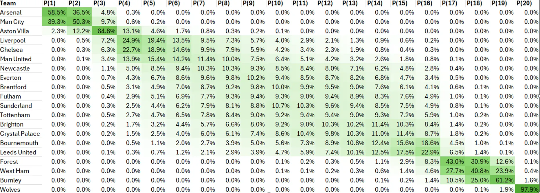
By calculating the expected number of goals that each team will score in each remaining match, we can sample Poisson random variables to simulate the rest of the season. We can then repeat the simulation many times and record the finishing position of each team in each simulation. Dividing the number of times a team finishes in a position by the total number of simulations run gives the probability of that team finishing in that position. The model can run 10,000 simulations in approximately 45 seconds, and this proved sufficient to produce stable probabilities.

The resulting output – as at the mid-point of the season – is shown below.

Limitations

There are a few limitations worth keeping in mind when reading the analysis below.

First, the model treats the two teams’ goal tallies as independent of one another. In reality there is some dependence — teams tend to sit back when ahead and push forward when losing — but the model does not account for this.

Second, the only data inputs are the actual numbers of goals scored and conceded in each match. This introduces noise into the predictions that a more sophisticated approach might reduce.

Third, the model takes no account of effects such as managerial changes, injuries to key players, January signings, fatigue from a busy schedule, or increased motivation from fighting for survival or for European qualification. Any of these could have a significant short-term impact — and as we’ll show, managerial changes in particular became a key factor in the Relegation Battle this season.

Title Race

Champions Liverpool started the season as the strongest side in the league, winning their first 5 games, including a narrow victory over potential title rivals Arsenal. At this stage my model gave them a 53% chance of retaining their crown. Arsenal and Tottenham led the chase, with Manchester City given only a 2% chance of recovering from their poor start.

However, Liverpool then lost 6 of their next 7 games, while Arsenal, Manchester City, and Chelsea began winning streaks of their own. This effectively ended Liverpool’s hopes of defending their title, while giving Arsenal a great chance to finally claim the Premier League trophy.

The title race ebbed and flowed but Arsenal maintained a strong position at the top of the table until the March international break. At this point they were 9 points ahead of Manchester City, who had played one fewer game. Arsenal’s remaining fixtures also looked more favourable on paper, and my model gave them a 97% chance of holding on.

However, a damaging home defeat to Bournemouth — while Manchester City won away at Chelsea — followed by a narrow defeat against Manchester City threw the title race wide open. After beating Burnley, City went top of the table, tied on points and goal difference but ahead on goals scored, with 5 games left each.

Most pundits expected City to push on and claim the title from here. My model gave Arsenal a narrow edge. Arsenal did go on to win the title.

Relegation Battle

Looking at the bottom of the table: by the midpoint of the season, both Burnley and Wolverhampton Wanderers had struggled so badly that my model gave each a roughly 90%+ chance of relegation. This left the final relegation spot to be fought over between West Ham, Nottingham Forest, and Leeds.

After losing at home to Forest in January, West Ham were left 7 points adrift. Their situation inspired a sharp improvement in form, and they quickly racked up 3 wins. Meanwhile, Tottenham’s results were deteriorating under manager Thomas Frank, and by the time he was sacked in mid-February they were being drawn into the relegation picture. New manager Igor Tudor took over, but 4 defeats in 5 games followed. West Ham continued their good form, and by the time Tottenham appointed their third manager, Roberto De Zerbi, in late February, my model had them marked as the most likely candidate for relegation. He was able to quickly turn things around, ultimately keeping Tottenham in the top flight at West Ham’s expense.

This is a good illustration of one of my model’s core limitations: it has no way to factor in the appointment of a new manager. But it’s worth noting that the impact of a managerial change is itself highly unpredictable — a new manager can transform a team’s fortunes, or as in this case make things worse. It is not clear that accounting for managerial changes would meaningfully improve a model’s accuracy, given how varied the outcomes tend to be.

Conclusion

The question this project set out to explore was how accurately it is possible to predict the Premier League season using a relatively simple model, built in nothing more powerful than Excel. Does it really take a supercomputer? The answer appears to be no – the model’s prediction for the title winner never swayed from Arsenal from November onwards, and it tracked the shifting probabilities of the relegation battle plausibly throughout the season.

Where it fell short is instructive. The model cannot predict the effect of managerial changes, and Tottenham’s turbulent season illustrated that limitation clearly. The model reflected Tottenham’s decline as it happened, but it couldn’t anticipate this dramatic change in fortunes ahead of time.

There is room to improve. Replacing raw goals data with expected goals (xG) — a measure of the quality of chances created and conceded, rather than just the outcomes — would likely reduce some of the noise in the predictions. Modelling some dependence between the two teams’ scores, and accounting for fixture congestion, would add further sophistication.

But the broader point stands: meaningful predictions are achievable without enormous computational power.

Tom Uden

May 2026